


Dependent Stress-Strength Reliability Model with Modified Weibull Distribution Marginals via Clayton Copula
This R package, SSReliabilityClaytonMWD, implements
dependent stress–strength reliability (SSR) model with Modified Weibull
marginals and a Clayton copula for dependence, based on the study by Kızılaslan (2026).
The package includes:
You can install the development version from GitHub:
# install.packages("remotes")
# remotes::install_github("fatihki/SSReliabilityClaytonMWD")
library(SSReliabilityClaytonMWD)The modified Weibull distribution (MWD), introduced by Lai et al. (2003), which has been widely used in reliability and survival analysis. A random variable \(X\) is said to follow a modified Weibull distribution if its cumulative distribution function (cdf) \(F(x)\) and probability density function (pdf) \(f(x)\) are given by \(F(x) = 1- \exp \big( -a x^b e^{\lambda x} \big)\) and \(f(x) = a (b + \lambda x) x^{b-1} e^{\lambda x} \exp \big( -a x^b e^{\lambda x} \big)\), where \(x>0\), \(a>0\) is the scale parameter, \(b \ge 0\) is a shape parameter, and \(\lambda \ge 0\) is an acceleration or flexibility parameter that controls how quickly the hazard grows over time. When \(\lambda=0\), it reduces to the two-parameter Weibull distribution with \(F(x) = 1- \exp(-a x^b)\). When \(b=0\), it reduces to a type I extreme-value (or log-gamma) distribution with \(F(x) = 1- \exp(-a e^{\lambda x} )\).
# Parameters
a1 <- 5; b1 <- 0.75; lambda1 <- 0.5
a2 <- 5; b2 <- 1.5; lambda2 <- 0.5

x <- seq(1e-02, 3, length.out = 1000)
# First curve
plot(x, dMweibull(x, a1, b1, lambda1),
type = "l", lwd = 2, lty = 1,
xlab = "x", ylab = "pdf",
main = "Modified Weibull Probability Density Function")
# Second curve
lines(x, dMweibull(x, a2, b2, lambda2),
lwd = 2, lty = 2)
# Legend
legend("topright",
legend = c(expression(b1==1.5), expression(b2==0.75)),
lty = c(1, 2),
lwd = 2, bty = "n")
plot(x, pMweibull(x, a1, b1, lambda1), type = "l", lwd = 2,  lty = 1,
     xlab = "x", ylab = "cdf",
     main = "Modified Weibull Cumulative Distribution Function")
# Second curve
lines(x, pMweibull(x, a2, b2, lambda2),
      lwd = 2, lty = 2)
# Legend
legend("topright",
       legend = c(expression(b1==1.5), expression(b2==0.75)),
       lty = c(1, 2),
       lwd = 2,  bty = "n")
plot(x, hMweibull(x, a1, b1, lambda1), type = "l", lwd = 2, lty = 1,
     xlab = "x", ylab = "hazard",  ylim = c(0,40),
     main = "Modified Weibull Hazard Function")
# Second curve
lines(x, hMweibull(x, a2, b2, lambda2),
      lwd = 2, lty = 2)
# Legend
legend("topleft",
       legend = c(expression(b1==1.5), expression(b2==0.75)),
       lty = c(1, 2),
       lwd = 2,  bty = "n")
a <- 0.75; b <- 1.25; lambda <- 0.6
set.seed(123)
X <- rMweibull(100, a, b, lambda)hist(X, breaks = 20, main = "Simulated MWD Data", xlab = "X")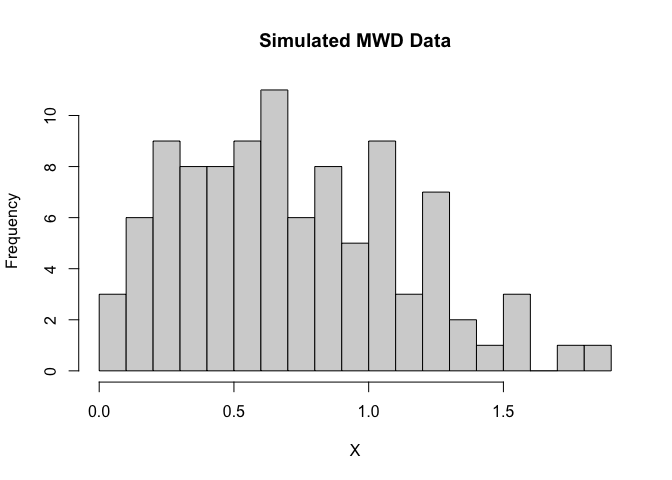
Estimation of MWD parameters using MLE, LSE, WLSE and MPS methods.
# Fit Modified Weibull Distribution
set.seed(123)
init <- runif(3)
fit.mle <- fitMWD( data = X, est.method = "mle", opt.method = "L-BFGS-B", starts = init,
  lower = c(1e-05, 1e-05, 1e-05), upper = c(Inf, Inf, Inf))
fit.lse <- fitMWD( data = X, est.method = "lse", opt.method = "L-BFGS-B", starts = init,
  lower = c(1e-05, 1e-05, 1e-05), upper = c(Inf, Inf, Inf))
fit.wlse <- fitMWD( data = X, est.method = "wlse", opt.method = "L-BFGS-B", starts = init,
  lower = c(1e-05, 1e-05, 1e-05), upper = c(Inf, Inf, Inf))
fit.mps <- fitMWD( data = X, est.method = "mps", opt.method = "L-BFGS-B", starts = init,
  lower = c(1e-05, 1e-05, 1e-05), upper = c(Inf, Inf, Inf))
# estimates results| a | b | lambda | |
|---|---|---|---|
| True | 0.75000 | 1.25000 | 0.60000 |
| MLE | 0.72316 | 1.26009 | 0.65591 |
| LSE | 0.92991 | 1.40695 | 0.40209 |
| WLSE | 0.92201 | 1.42281 | 0.42073 |
| MPS | 0.71406 | 1.18911 | 0.64607 |
Similarly, the two-parameter Weibull distribution can be also fitted
to data bySSReliabilityClaytonMWD::fitWD.
The stress–strength reliability \(R = P(X > Y)\) under a dependent framework, where both stress \(X\) and strength \(Y\) variables follow MWD and their dependence is modeled via a Clayton copula.
The joint distribution function of the two-dimensional Clayton copula, along with its joint probability density function, are given by \(C_{\theta}(u,v) = (u^{-\theta} + v^{-\theta} - 1)^{-1/\theta}\) and \(c_{\theta}(u,v) = (\theta +1) u^{-(\theta + 1)} v^{-(\theta + 1)} \big( u^{-\theta} + v^{-\theta}-1 \big)^{-\left (\frac{1}{\theta} + 2 \right)}\), where \(\theta >0\). When \(X \sim MWD(a_1,b_1,\lambda_1)\), \(Y \sim MWD(a_2,b_2,\lambda_2)\) with the two-dimensional Clayton copula from, \(R\) becomes \(R = \int_{0}^{\infty} F_X(x)^{-(\theta + 1)} \big(F_X(x)^{-\theta} + G_Y(x)^{-\theta}-1 \big) ^{-\left (\frac{1}{\theta}+1 \right)} f_X(x) \mathrm{d}x = \int_{0}^{1} t^{-(\theta +1)} \big( t^{-\theta} + G_Y(F_{X}^{-1}(t))^{-\theta} -1 \big)^ {-\left(\frac{1}{\theta}+1 \right) } \mathrm{d}t\), where \(F_X(x) \equiv F_X(x;a_1,b_1,\lambda_1) = 1- \exp(-a_1 x^{b_1} e^{\lambda_1 x})\) and \(G_Y(y) \equiv G_Y(y;a_2,b_2,\lambda_2) = 1- \exp(-a_2 y^{b_2} e^{\lambda_2 y})\).
The applicability of the proposed SSR model is illustrated using monthly occupancy data from Istanbul’s two largest dams, with the Clayton copula capturing their dependence structure.
The data is obtained from open data platform of the Istanbul Metropolitan Municipality https://data.ibb.gov.tr/en/. The dataset consists of daily occupancy rates of Istanbul’s dams, retrieved in March 2026 from data-website.
In this study, we focus on the two largest dams: Omerli (Anatolian
side) and Terkos (European side). The data span the period from late
October 2000 to mid-February 2024. To reduce variability and focus on
seasonal effects, we compute monthly average occupancy rates for the
period September–December of each year. This results in a total of 95
paired observations for both variables. The used Omerli and Terkos dams
data are available in this package as OmerliDam and
TerkosDam. Additionally, the daily occupancy rates data of
all Istanbul’s dams for the same period is available in this package as
AllDams.
In the stress–strength framework, the Terkos dam is treated as the strength variable \(X\), while the Omerli dam is considered as the stress variable \(Y\). Under this formulation, the SSR \(R=P(X>Y)\) represents the probability that the occupancy level of the Terkos dam (European side) exceeds that of the Omerli dam (Anatolian side). This probability quantifies the likelihood that local water availability on the European side is sufficient relative to the corresponding level on the Anatolian side. In practical terms, when the Terkos level falls below that of Omerli, additional water transfer to the European side may be required. A higher value of \(R\) indicates a more favorable scenario, implying a reduced need for water transfer and lower operational costs, whereas lower values of \(R\) suggest increased reliance on inter-regional water transfer and, consequently, higher system costs and risks. Further details can be found in Kızılaslan (2026).
Fitting the dependent SSR model with a Clayton copula and Modified Weibull distributions to the Omerli and Terkos dam occupancy data, as presented in Table 7 of Kızılaslan (2026).
data <- list(X = TerkosDam, Y = OmerliDam)

fit <- fit.SSR.ClaytonMWD(
  data,
  ACI = TRUE,
  bootstrap = TRUE,
  B = 10,
  seed = 2026,
  one.step = TRUE,
  alpha = 0.05
)
#> Warning: executing %dopar% sequentially: no parallel backend registered

print(fit)
#>
#> Fitting Results of Stress-Strength Reliability Model with MWD Marginals via Clayton Copula
#>
#>
#> Table: Parameter Estimates
#>
#> |     |      a1|      b1| lambda1|      a2|      b2| lambda2|   theta|       R|
#> |:----|-------:|-------:|-------:|-------:|-------:|-------:|-------:|-------:|
#> |mle  | 0.98542| 2.66095| 2.11322| 0.02428| 0.45908| 6.33059| 0.50551| 0.50428|
#> |lse  | 0.07196| 1.72091| 5.71667| 0.01166| 0.00001| 7.06623| 1.09884| 0.49349|
#> |wlse | 0.04261| 1.29079| 6.20629| 0.01154| 0.00001| 7.10656| 1.23631| 0.49824|
#> |mps  | 0.68997| 2.31111| 2.39000| 0.02043| 0.26258| 6.43699| 0.92547| 0.51110|
#>
#>
#> Table: 95% Asymptotic Confidence Intervals (MLE)
#>
#> |       |      a1|      b1| lambda1|      a2|      b2| lambda2|   theta|       R|
#> |:------|-------:|-------:|-------:|-------:|-------:|-------:|-------:|-------:|
#> |lower  | 0.00000| 0.43992| 0.00000| 0.00000| 0.00000| 4.21722| 0.14734| 0.40310|
#> |upper  | 4.33682| 4.88197| 5.79639| 0.06723| 1.39756| 8.44395| 0.86369| 0.60545|
#> |length | 4.33682| 4.44205| 5.79639| 0.06723| 1.39756| 4.22673| 0.71636| 0.20235|
#>
#>
#> Table: 95% Bootstrap CIs (MLE)
#>
#> |       |      a1|      b1| lambda1|     a2|      b2| lambda2|   theta|       R|
#> |:------|-------:|-------:|-------:|------:|-------:|-------:|-------:|-------:|
#> |lower  | 0.08013| 1.15190| 0.00001| 0.0127| 0.14660| 2.96074| 0.24032| 0.44208|
#> |upper  | 7.84406| 4.17488| 4.99832| 0.6515| 2.74715| 7.36907| 0.76629| 0.57280|
#> |length | 7.76393| 3.02298| 4.99831| 0.6388| 2.60056| 4.40833| 0.52597| 0.13072|
#>
#>
#> Table: 95% Bootstrap CIs (LSE)
#>
#> |       |       a1|      b1| lambda1|      a2|      b2| lambda2|   theta|       R|
#> |:------|--------:|-------:|-------:|-------:|-------:|-------:|-------:|-------:|
#> |lower  |  0.00432| 0.00001| 0.08203| 0.00479| 0.00001| 3.38092| 0.77300| 0.40633|
#> |upper  | 14.07044| 5.07941| 8.83643| 0.46871| 2.90343| 8.70306| 1.22167| 0.54812|
#> |length | 14.06612| 5.07940| 8.75439| 0.46392| 2.90342| 5.32214| 0.44867| 0.14178|
#>
#>
#> Table: 95% Bootstrap CIs (WLSE)
#>
#> |       |      a1|      b1| lambda1|      a2|      b2| lambda2|   theta|       R|
#> |:------|-------:|-------:|-------:|-------:|-------:|-------:|-------:|-------:|
#> |lower  | 0.00600| 0.08335| 2.07582| 0.00735| 0.00001| 4.57432| 1.02051| 0.40990|
#> |upper  | 1.93694| 3.81682| 8.40554| 0.14362| 2.18957| 7.75921| 2.79450| 0.55191|
#> |length | 1.93094| 3.73347| 6.32972| 0.13627| 2.18956| 3.18489| 1.77400| 0.14201|
#>
#>
#> Table: 95% Bootstrap CIs (MPS)
#>
#> |       |      a1|      b1| lambda1|      a2|      b2| lambda2|   theta|       R|
#> |:------|-------:|-------:|-------:|-------:|-------:|-------:|-------:|-------:|
#> |lower  | 0.03681| 0.81306| 0.20976| 0.00853| 0.00001| 3.89184| 0.39588| 0.43467|
#> |upper  | 4.90435| 3.55720| 5.68968| 0.23335| 1.80479| 7.53494| 5.25280| 0.62724|
#> |length | 4.86754| 2.74414| 5.47992| 0.22482| 1.80478| 3.64310| 4.85692| 0.19257|
#>
#> Kendall's tau estimate for theta: 1.25912Kızılaslan, Fatih. (2026). Reliability estimation in dependent stress–strength model with Clayton copula and modified Weibull margins.arXiv:2604.12130
Lai, C. D., Xie, M., & Murthy, D. N. P. (2003). A modified Weibull distribution. IEEE Transactions on Reliability, 52(1), 33–37. doi.org/10.1109/TR.2002.805788
This package includes data obtained from Istanbul Metropolitan Municipality Open Data Portal. The data have been formatted for use within this package. All rights to the original data belong to the data provider.