Spotted arrays print-run quality control

April 15, 2008

Agnes Paquet¹, Andrea Barczak¹, (Jean) Yee Hwa Yang²

1. Department of Medicine, Functional Genomics Core Facility, University of California, San Francisco
paquetagnes@yahoo.com
2. School of Mathematics and Statistics, University of Sydney, Australia

Content

1. Print-run quality control

When a print-run is completed, it is necessary to verify the quality of the resulting arrays. This can be done by using two kinds of hybridization to the new slides. The first type of hybridization, which we term “9mers hyb”, uses small oligonucleotides (random 9-mers), which will hybridize to each probe. This hybridization will help to determine the quality of spot morphology as well as the presence or absence of spotted oligonucleotides. The resulting data will be used to create a list of all missing spots.

The second type of hybridization, which we will term Quality Control Hybridization (QCHyb), uses mRNA from predefined cell lines (e.g. liver vs. pool, K562 vs. Human Universal Reference pool from Stratagene). These hybridizations can be use as a more quantitative description of the slides. The same comparison hybridizations are done for different print-run, assessing their reproducibility. QCHybs are also used to verify accuracy of GAL files, number of missing spots, binding capacity, background signal intensity…

The arrayQuality package provides specific tools to help assess quality of slides for both 9-mers and QC hybridization.

2. 9-mers hybridizations

• Copy all 9-mers hybridizations gpr files from the SAME print-run (same GAL file) to a directory.
• Change R working directory to the one containing your gpr files using the R GUI menu.
• To load arrayQuality:
  Type at the R prompt:
  library(arrayQuality)
  
• To run th function type:
  PRv9mers(prname=”12Mm”).

2.1 Results

1. Diagnostic plots as image in .png format for each tested slide


2. An Excel file (typically named 9Mm9mer.xls, where 9Mm is the name of your print-run, as passed to prname) containing for each spot on the slide:
   
   • Name and ID of the spot
   • The probability of being present or absent (p from EM algorithm). If several files are tested together, you will have a probability of being present/absent for each file.
     A spot is considered absent if p < 0.5.
   • The average probability of being present or absent.
   • The raw signal intensity (Signal column) or average raw signal intensity if several files are tested together for each spot.
3. An Excel file (typically named 9MmMissing.xls, where 9Mm is the name of your print-run, as passed to prname) containing information on missing probes only:
   
   • Name and ID of the spot
   • The probability of being present or absent (p from EM algorithm). If several files are tested together, you will have a probability of being present/absent for each file.
     A spot is considered absent if p < 0.5.
   • The average probability of being present or absent.
   • The raw signal intensity (Signal column) or average raw signal intensity if several files are tested together for each spot.


4. A text file (typically named 9MmQuickList.txt, where 9Mm is the name of your print-run, as passed to prname) containing the missing probes ids, each on a separate line. This file can be opened in any word processing program.

2.2 Description of the diagnostic plots

1. The first column (left) represents boxplots of log intensity, by plates (top) and by print-tip group (bottom). In this example, you will notice on the boxplot by plates (top left corner) that plates 44 and 48 have lower intensity and wider range than the others. Both plates contain mostly empty controls, as designed by Operon.
2. Central plot: spatial plot of intensity. This helps to locate missing spots. The color scale reflects the signal intensity, the darker the color of the plot, the stronger the signal. Missing spots are represented in white. In Figure 3 spatial plot, top right corner white spots come from the empty spots.
3. Right column: Density plot of the foreground and background log intensity.
   1. Foreground density plot: it should be composed of 2 peaks. A smaller peak in the low intensity region containing missing spots and negative control spots, and a higher one representing the rest of the spots (probes). The number of present and absent spots, excluding empty controls, estimated by EM algorithm is indicated on the graph.
   2. Background density plot: one peak in the low intensity region. If a slide is of good quality, the background peak should not overlap too much with the foreground peak corresponding to the bulk of the data.

2.3 Examples

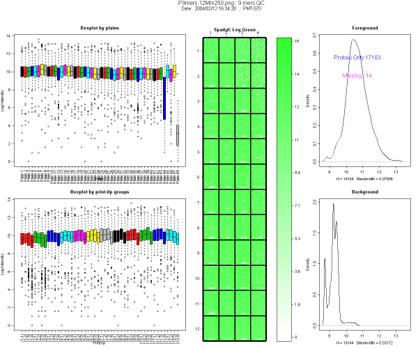
Figure 1: Example of diagnostic plot for 9-mers hybridization

3. Quality Control hybridizations

9-mers hybridizations help verify that oligonucleotides have been spotted properly on the slides. The next print-run quality control step will be:

1.      Detect any difference in overall signal intensity compared to other print-runs

a.      70-mers oligonucleotides hybridizations

b.      Selection of several test slides to ensure that the same quantity of material was spotted across the platter, as a print-run will generate 255 slides using the same well for one probe. QCHybs are performed using one slide from the beginning of the print, one from the middle, one from the end (e.g. numbers 20,100 and 255 in the Functional Genomics Core Facility).

2.      Check if the GAL file was generated properly, i.e. check that no error was made with ordering or orientation of the plates during the print.

3.      Reproducibility:
A good way to verify the quality of a new print is to hybridize known samples to new slides. Then, we can compare signal intensity from the new slides to existing data, and check that there is no loss in signal. Log ratios (M) for known samples should be similar across print-runs. Example of samples used for QCHybs includes Human Reference pool, Mouse liver, Mouse lung, with dye swaps.

The function in the package which performs the quality assessment for QCHybs is PRvQCHyb(). It runs using a single line script. To use it:

• Copy the QCHybs gpr files from the SAME print-run (same GAL file) in a directory.
• Change R working directory to the one containing your gpr files as described in section 1.
•  Type in R: 

where prname is the name of the print-run. For more details about its arguments, please refer to the online manual.
 

3.1 Results 

PRvQCHyb() returns a diagnostic plot as an image in .png format for each tested slide.

Throughout our document, we will be using the color code described in Table 1 to highlight control spots.

Table 1: Color code used in arrayQuality

Restrictions:

Currently, PRQCHyb() supports Mouse genome (Mm) only.  

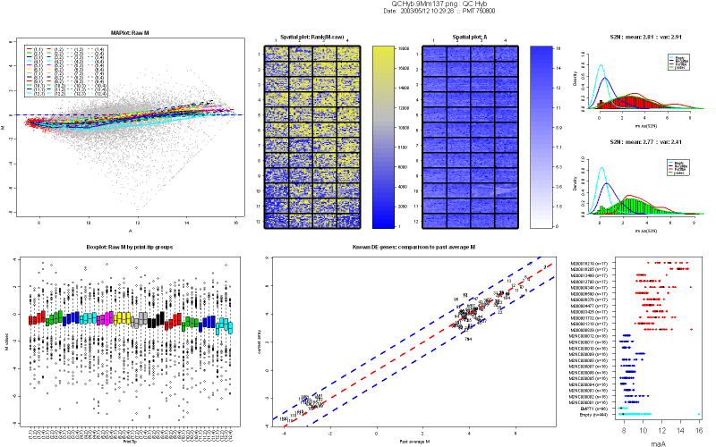
3.2 Description of the diagnostic plots

1. MA-plot of raw M values. No background subtraction is performed. The colored lines represent the loess curves for each print-tip group. The red dots highlight  any spot with corresponding weighted value  less than 0. Users can create their own weigthing scheme or function. Things to look for in a MA-plot are saturation of spots and the trend of loess curves, which is an indicator of the amount of normalization to be performed.
   

2. Boxplot of raw M values by print-tip group, without background subtraction.

3. Spatial plot of rank of raw M values (no background subtraction): Each spot is ranked according to its M value. We use a blue to yellow color scale,where blue represents the higher rank (1), and yellow represents the lower one. Missing spots are represented as white squares.

4. Spatial plot of A values. The color indicates the strength of the signal intensity, i.e. the darker the color, the stronger the signal. Missing spots are represented in white.

5. Histogram of the signal-to-noise log-ratio (SNR) for Cy5 and Cy3 channels. The mean and the variance of the signal are printed on top of the histogram. In addition, overlay density of SNR stratified by different control types (status) are highlighted. Their color schemes are provided in Table 1. The SNR is a good indicator for dye problems. The negative controls and empty controls density lines should be closer, almost superimposed.

6. Comparison of Mvalues of probes known to be differentially expressed from the tested array to average Mvalues obtained during previous hybridizations. This plot is aimed at verifying the reproducibility of print-runs. The dotted lines are the diagonal (no change) and the +2/-2 fold change lines. Each probe is represented by a number, and described in the file MmDEGenes.xls. Most of the spots should lie between the +2/-2 fold-change regions. If the technique was perfect, you should see a straight line on the diagonal. If any probe falls off this region (number 29 here), you can look up its number in our probe list in MmDEgenes.xls and get more information about it.

7. Dot plot of controls A values, without background subtraction. Controls with more than 3 replicates are represented on the Y-axis, the color scheme is represented in Table 1. Intensity of positive controls should be in the high-intensity region, negative and empty controls should be in the lower intensity region. Positive controls range and negative/empty controls range should be separated. Replicate spots signal should be tight.
   

3.3 Example

Data for this example was provided by the Functional Genomics Core Facility in UCSF. We have tested slide number 137 from print-run 9Mm. This print-run uses Operon Version 2 Mouse oligos. Results are represented figure 2. 

> library(arrayQuality)

> datadir <- system.file("gprQCData", package="arrayQuality")

> PRvQCHyb(fnames=”9Mm137.gpr”, path=datadir, prname="9Mm")

Figure 2: Diagnostic plot for print-run Quality Control hybridization