
![]()
![]()
![]()
![]()
![]()
![]()
![]()
The maxbootR package provides fast and
consistent bootstrap methods for block maxima, designed for
applications in extreme value statistics. Under the hood,
performance-critical parts are implemented in C++ via Rcpp, enabling
efficient computation even for long time series.
These methods are based on the first consistent bootstrap approach for block maxima as introduced in Bücher & Staud (2024+): Bootstrapping Estimators based on the Block Maxima Method..
You can install the development version of maxbootR from
GitHub with:
# install.packages("devtools")
devtools::install_github("torbenstaud/maxbootR")
or from the official CRAN repository in R with:
install.packages("maxbootR")The following example demonstrates how to extract sliding block maxima from synthetic data.
library(ggplot2)
library(maxbootR)
library(dplyr)

# Generate 100 years of daily observations
set.seed(91)
x <- rnorm(100 * 365)

# Extract sliding block maxima with 1-year window
bms <- blockmax(xx = x, block_size = 365, type = "sb")

# Create time-indexed tibble for plotting
df <- tibble(
  day = seq.Date(from = as.Date("1900-01-01"), by = "1 day", length.out = length(bms)),
  block_max = bms
)

# Plot the block maxima time series
ggplot(df, aes(x = day, y = block_max)) +
  geom_line(color = "steelblue") +
  labs(
    title = "Sliding Block Maxima from Simulated Data",
    x = "Year",
    y = "Block Maximum"
) 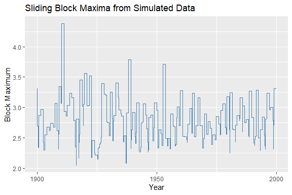
Time series of block maxima from simulated normal data
We now use the maxbootr() function to bootstrap the
100-year return level of synthetic data, comparing the
disjoint vs. sliding block bootstrap methods.
# Set block size (e.g., summer days)
bsize <- 92

# Generate synthetic time series
set.seed(1)
y <- rnorm(100 * bsize)

# Bootstrap using disjoint blocks (+timing)
system.time(
  bst.db <- maxbootr(xx = y, est = "rl", block_size = bsize, B = 500,
                     type ="db", annuity = 100)
)
#>        User      System verstrichen
#>        0.61        0.00        0.69

# Bootstrap using sliding blocks (+timing)
system.time(
  bst.sb <- maxbootr(xx = y, est = "rl", block_size = bsize, B = 500,
                     type = "sb", annuity = 100)
)
#>        User      System verstrichen
#>        6.86        0.00        6.89

# Compare variance
var(bst.sb) / var(bst.db)
#>           [,1]
#> [1,] 0.5502442
The sliding block method typically results in narrower bootstrap distributions, reducing statistical uncertainty.
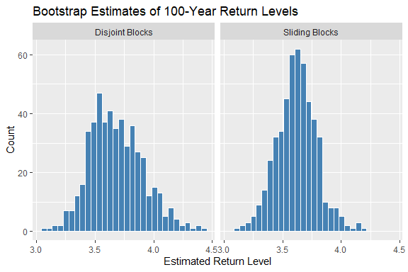
Histogram of return level bootstrap replicates
For a full tutorial with real-world case studies (finance & climate), check out the vignette included in the package.
The implemented disjoint and sliding block bootstrap methods are grounded in the following foundational works:
The block bootstrap methodology itself is based on:
I plan to further enhance maxbootR by:
Your ideas and contributions are welcome — feel free to open an issue or pull request on GitHub!