footBayes

The goal of footBayes is to propose a complete workflow to:

• Fit the most well-known football models, including the double Poisson, bivariate Poisson, Dixon-Coles, negative binomial, Skellam, Student-t, diagonal-inflated bivariate Poisson and zero-inflated Skellam distributions. It supports both maximum likelihood estimation (MLE) and Bayesian inference. For Bayesian methods, it incorporates several techniques: MCMC sampling with Hamiltonian Monte Carlo, variational inference using either the Pathfinder algorithm or Automatic Differentiation Variational Inference (ADVI), and the Laplace approximation.

• Model static or dynamic team abilities (weekly or seasonal), choosing among alternative evolution variances: separate attack/defence variances (Egidi et al., 2018), a common variance (Owen, 2011), variance inflation after the summer break (Koopman and Lit, 2015), and the weighted dynamic models with commensurate priors (Macrì Demartino, Egidi and Torelli, 2026).

• Estimate historical team strengths with a Bayesian Bradley-Terry-Davidson model and use them as a covariate in the goal-based models.

• Visualize the teams’ abilities, the model checks, the rank-league reconstruction;

• Predict out-of-sample matches and compare models through predictive metrics.

Installation

Starting with version 2.0.0, footBayes package requires installing the R package cmdstanr (not available on CRAN) and the command-line interface to Stan: CmdStan. For a step-by-step installation, please follow the instructions provided in Getting started with CmdStanR.

You can install the released version of footBayes from CRAN with:

install.packages("footBayes", type = "source")

Please note that it is important to set type = "source". Otherwise, the ‘CmdStan’ models in the package may not be compiled during installation.

Alternatively to CRAN, you can install the development version from GitHub with:

# install.packages("devtools")
devtools::install_github("leoegidi/footBayes")

Example

In what follows, a quick example to fit a Bayesian double Poisson model for the Italian Serie A (seasons 2000-2001, 2001-2002, 2002-2003), visualize the estimated teams’ abilities, and predict the last four match days for the season 2002-2003:

library(footBayes)
library(dplyr)

# Dataset for Italian Serie A
data("italy")
italy <- as_tibble(italy)
italy_2000_2002 <- italy %>%
  dplyr::select(Season, home, visitor, hgoal, vgoal) %>%
  filter(Season == "2000" | Season == "2001" | Season == "2002")

colnames(italy_2000_2002) <- c("periods",
                               "home_team",
                               "away_team",
                               "home_goals",
                               "away_goals")

# Double poisson fit (predict last 4 match-days)
fit1 <- stan_foot(data = italy_2000_2002,
                  model = "double_pois",
                  predict = 36,
                  iter_sampling = 200,
                  chains = 2) 

The results (i.e., attack and defense effects) can be investigated using

print(fit1, pars = c("att", "def"))

To visually investigate the attack and defense effects, we can use the foot_abilities function

foot_abilities(fit1, italy_2000_2002) # teams abilities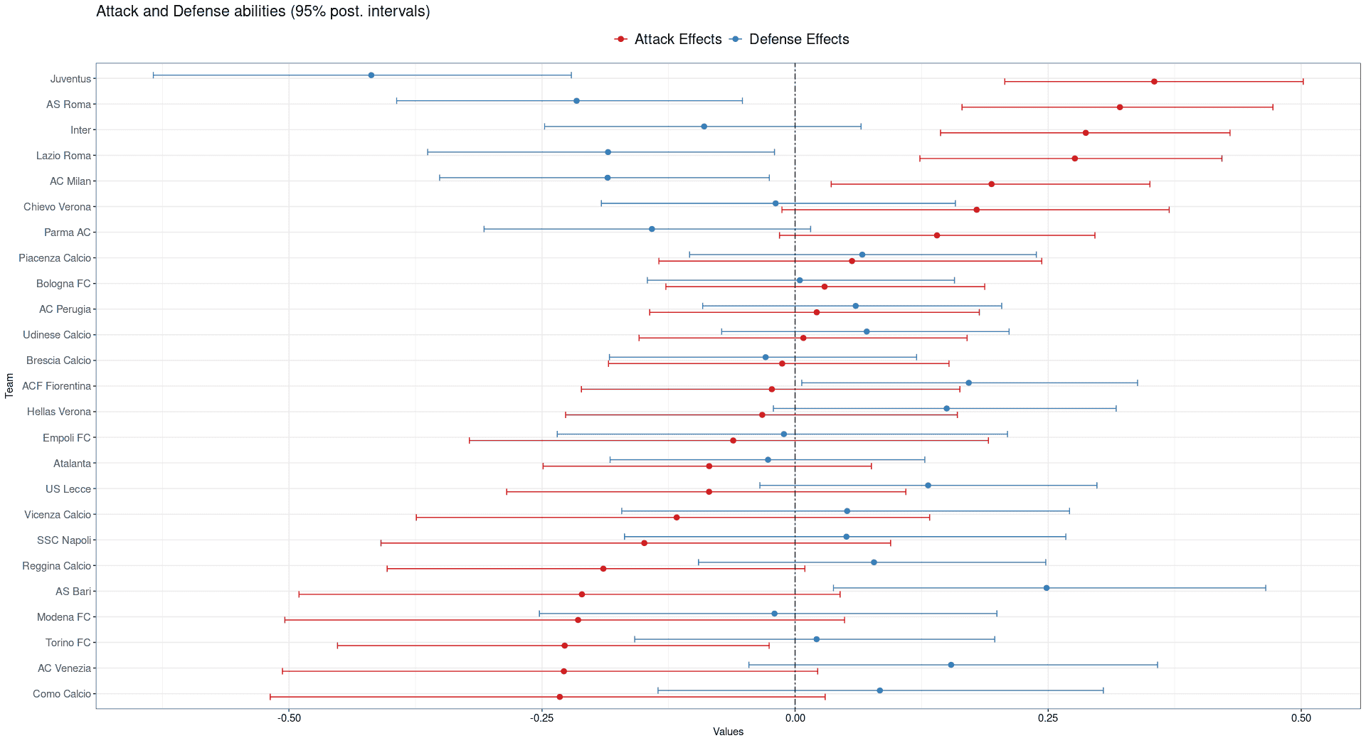

To check the adequacy of the Bayesian model the function pp_foot provides posterior predictive plots

pp_foot(fit1, italy_2000_2002) # pp checks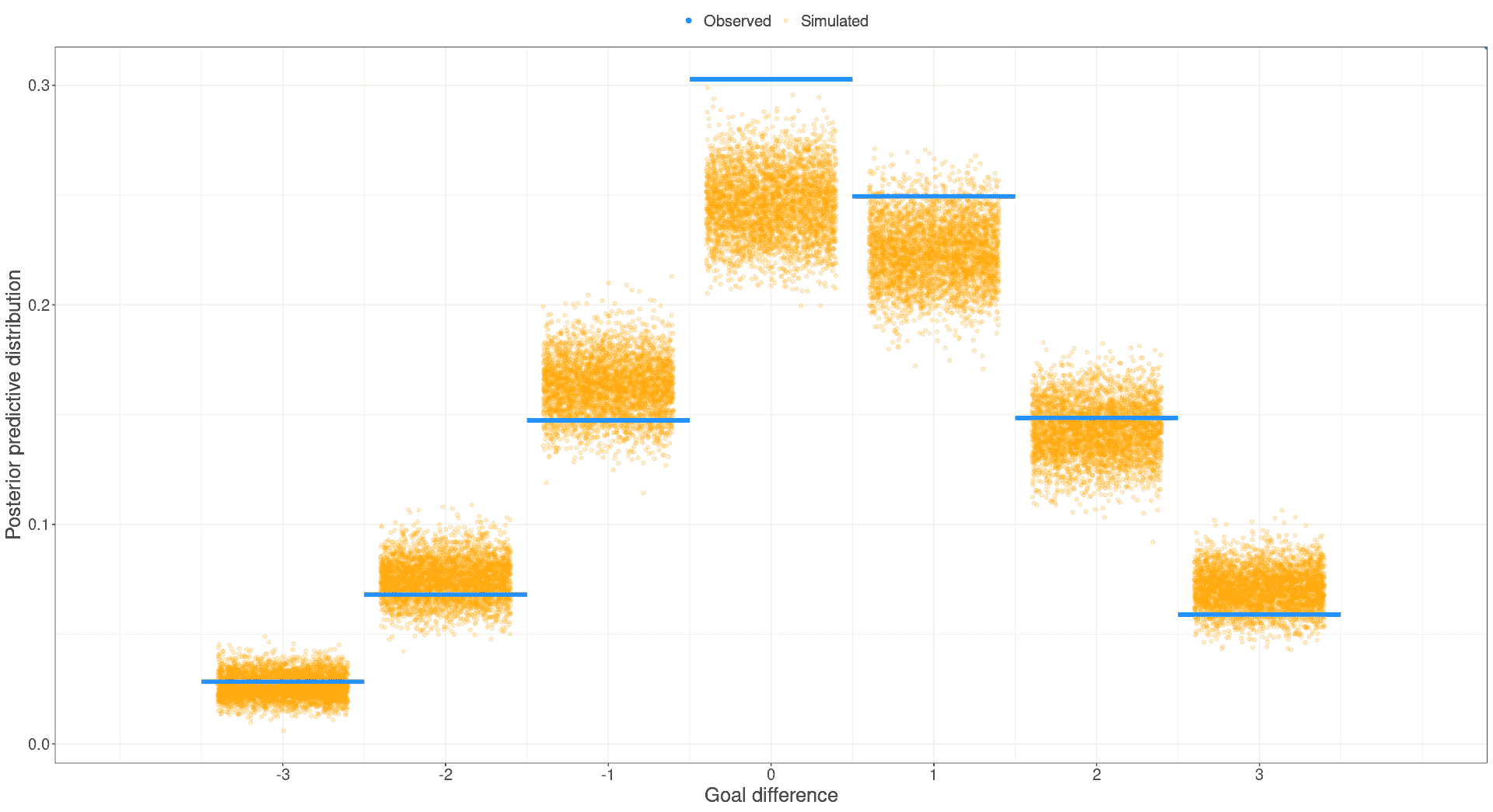

Furthermore, the function foot_rank shows the final rank table and the plot with the predicted points

foot_rank(fit1, italy_2000_2002) # rank league reconstruction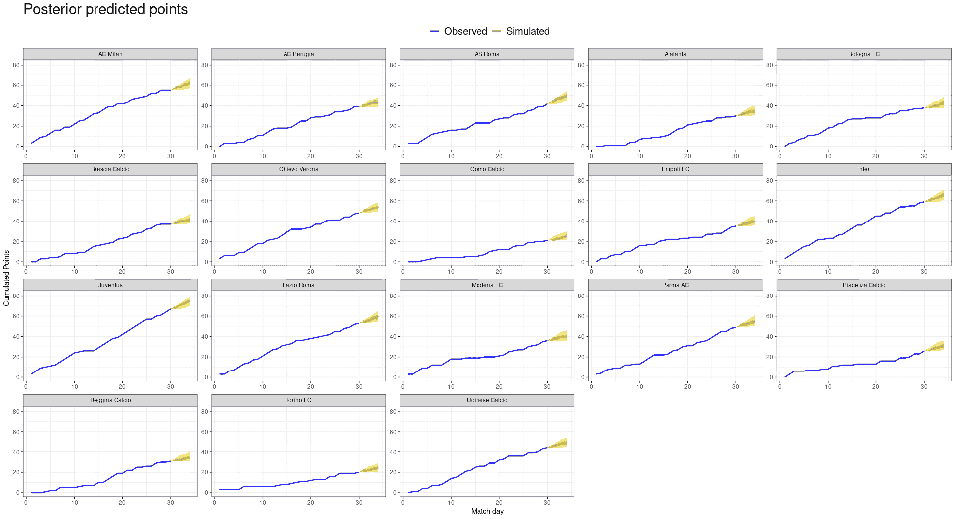

In order to analyze the possible outcomes of the predicted matches, the function foot_prob provides a table containing the home win, draw and away win probabilities for the out-of-sample matches

foot_prob(fit1, italy_2000_2002) # out-of-sample posterior pred. probabilities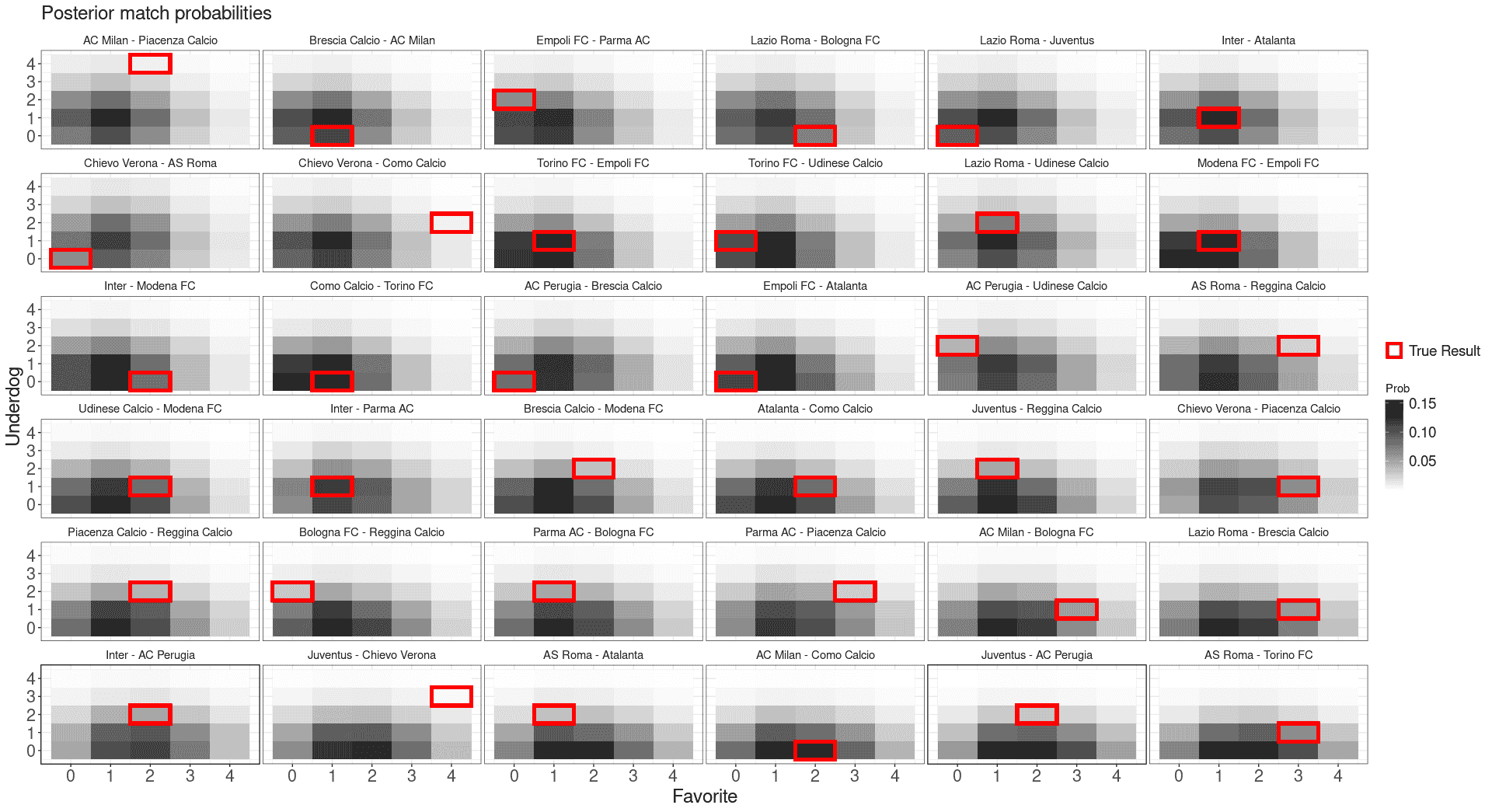

For more and more technical details and references, see the vignette!