![]()
![]()
![]()
Efficient approximate Bayesian inference for Structural Equation Models.
While Markov Chain Monte Carlo (MCMC) methods remain the gold
standard for exact Bayesian inference, they can be prohibitively slow
for iterative model development. {INLAvaan} offers a rapid
alternative for latent
variable analysis,
delivering Bayesian results at (or near) the speed of frequentist
estimators. It achieves this through a custom, ground-up implementation
of the Integrated Nested Laplace
Approximation (INLA), engineered specifically for the lavaan modelling framework.
{INLAvaan} is designed to fit seamlessly into your
existing workflow. If you are familiar with the (b)lavaan
syntax, you can begin using {INLAvaan} immediately.
As a first impression of the package, consider the canonical example of SEM applied to the Industrialisation and Political Democracy data set of Bollen (1989)1:
library(INLAvaan)
model <- "
  # Latent variable definitions
     ind60 =~ x1 + x2 + x3
     dem60 =~ y1 + y2 + y3
     dem65 =~ y5 + y6 + y7 + y8

  # Latent regressions
    dem60 ~ ind60
    dem65 ~ ind60 + dem60

  # Residual correlations
    y1 ~~ y5
    y2 ~~ y4 + y6
    y3 ~~ y7
    y4 ~~ y8
    y6 ~~ y8

  # Fixed loading
    dem60 =~ 1.5*y4

  # Custom priors on latent variances
    ind60 ~~ prior('gamma(1, 1)')*ind60
    dem60 ~~ prior('gamma(2, 1)')*dem60
    dem65 ~~ prior('gamma(1,.5)')*dem65
"
utils::data("PoliticalDemocracy", package = "lavaan")

fit <- asem(model, PoliticalDemocracy)
#> ℹ Finding posterior mode.
#> ✔ Finding posterior mode. [35ms]
#>
#> ℹ Computing the Hessian.
#> ✔ Computing the Hessian. [92ms]
#>
#> ℹ Performing VB correction.
#> ✔ VB correction; mean |δ| = 0.035σ. [84ms]
#>
#> ⠙ Fitting skew normal to 0/30 marginals.
#> ⠹ Fitting skew normal to 6/30 marginals.
#> ⠸ Fitting skew normal to 18/30 marginals.
#> ⠼ Fitting skew normal to 29/30 marginals.
#> ✔ Fitting skew normal to 30/30 marginals. [549ms]
#>
#> ℹ Sampling covariances and defined parameters.
#> ✔ Sampling covariances and defined parameters. [59ms]
#>
#> ⠙ Computing ppp and DIC.
#> ⠹ Computing ppp and DIC.
#> ✔ Computing ppp and DIC. [192ms]
#>

summary(fit)
#> INLAvaan 0.2.3 ended normally after 80 iterations
#>
#>   Estimator                                      BAYES
#>   Optimization method                           NLMINB
#>   Number of model parameters                        30
#>
#>   Number of observations                            75
#>
#> Model Test (User Model):
#>
#>    Marginal log-likelihood                   -1651.231
#>    PPP (Chi-square)                              0.170
#>
#> Information Criteria:
#>
#>    Deviance (DIC)                             3214.887
#>    Effective parameters (pD)                    58.157
#>
#> Parameter Estimates:
#>
#>    Marginalisation method                     SKEWNORM
#>    VB correction                                  TRUE
#>
#> Latent Variables:
#>                    Estimate       SD     2.5%    97.5%     NMAD    Prior
#>   ind60 =~
#>     x1                1.000
#>     x2                2.213    0.145    1.945    2.515    0.006    normal(0,10)
#>     x3                1.847    0.156    1.552    2.166    0.006    normal(0,10)
#>   dem60 =~
#>     y1                1.000
#>     y2                1.443    0.168    1.118    1.777    0.001    normal(0,10)
#>     y3                1.168    0.155    0.868    1.478    0.001    normal(0,10)
#>   dem65 =~
#>     y5                1.000
#>     y6                1.260    0.188    0.921    1.659    0.012    normal(0,10)
#>     y7                1.362    0.175    1.042    1.731    0.022    normal(0,10)
#>     y8                1.384    0.182    1.056    1.770    0.023    normal(0,10)
#>   dem60 =~
#>     y4                1.500
#>
#> Regressions:
#>                    Estimate       SD     2.5%    97.5%     NMAD    Prior
#>   dem60 ~
#>     ind60             1.379    0.348    0.706    2.069    0.001    normal(0,10)
#>   dem65 ~
#>     ind60             0.524    0.234    0.073    0.991    0.001    normal(0,10)
#>     dem60             0.885    0.106    0.688    1.103    0.020    normal(0,10)
#>
#> Covariances:
#>                    Estimate       SD     2.5%    97.5%     NMAD    Prior
#>  .y1 ~~
#>    .y5                0.330    0.410    0.132    1.739    0.006       beta(1,1)
#>  .y2 ~~
#>    .y4                0.216    0.675   -0.134    2.517    0.004       beta(1,1)
#>    .y6                0.348    0.748    0.851    3.789    0.010       beta(1,1)
#>  .y3 ~~
#>    .y7                0.224    0.658   -0.207    2.378    0.005       beta(1,1)
#>  .y8 ~~
#>    .y4                0.069    0.448   -0.538    1.218    0.004       beta(1,1)
#>  .y6 ~~
#>    .y8                0.309    0.579    0.252    2.520    0.005       beta(1,1)
#>
#> Variances:
#>                    Estimate       SD     2.5%    97.5%     NMAD    Prior
#>     ind60             0.455    0.089    0.308    0.654    0.003      gamma(1,1)
#>    .dem60             3.121    0.602    2.109    4.458    0.000      gamma(2,1)
#>    .dem65             0.340    0.196    4.237    0.059    0.043     gamma(1,.5)
#>    .x1                0.088    0.021    0.196    0.053    0.007 gamma(1,.5)[sd]
#>    .x2                0.124    0.065    1.503    0.019    0.040 gamma(1,.5)[sd]
#>    .x3                0.500    0.098    0.337    0.718    0.003 gamma(1,.5)[sd]
#>    .y1                2.311    0.490    3.406    1.495    0.004 gamma(1,.5)[sd]
#>    .y2                7.504    1.414   10.634    5.114    0.003 gamma(1,.5)[sd]
#>    .y3                5.500    1.063    3.733    7.883    0.002 gamma(1,.5)[sd]
#>    .y5                2.627    0.541    3.836    1.724    0.005 gamma(1,.5)[sd]
#>    .y6                5.132    0.947    3.529    7.227    0.003 gamma(1,.5)[sd]
#>    .y7                3.610    0.771    5.332    2.324    0.008 gamma(1,.5)[sd]
#>    .y8                3.210    0.718    4.794    1.988    0.006 gamma(1,.5)[sd]
#> .y4 2.872 0.747 7.211 1.607 0.009 gamma(1,.5)[sd]Computation speed is valuable only when accuracy is preserved. Our
method yields posterior distributions that are visually and numerically
comparable to those obtained via MCMC (e.g., via
{blavaan}/Stan), but at a fraction of the computational
cost.
The figure below illustrates the posterior density overlap for the example above. The percentages refer to the one minus the Jensen-Shannon distance, which gives a measure of similarity between two probability distributions.
# install.packages("blavaan")
library(blavaan)
fit_blav <- bsem(model, PoliticalDemocracy)
res <- INLAvaan:::compare_mcmc(fit_blav, INLAvaan = fit)
print(res$p_compare)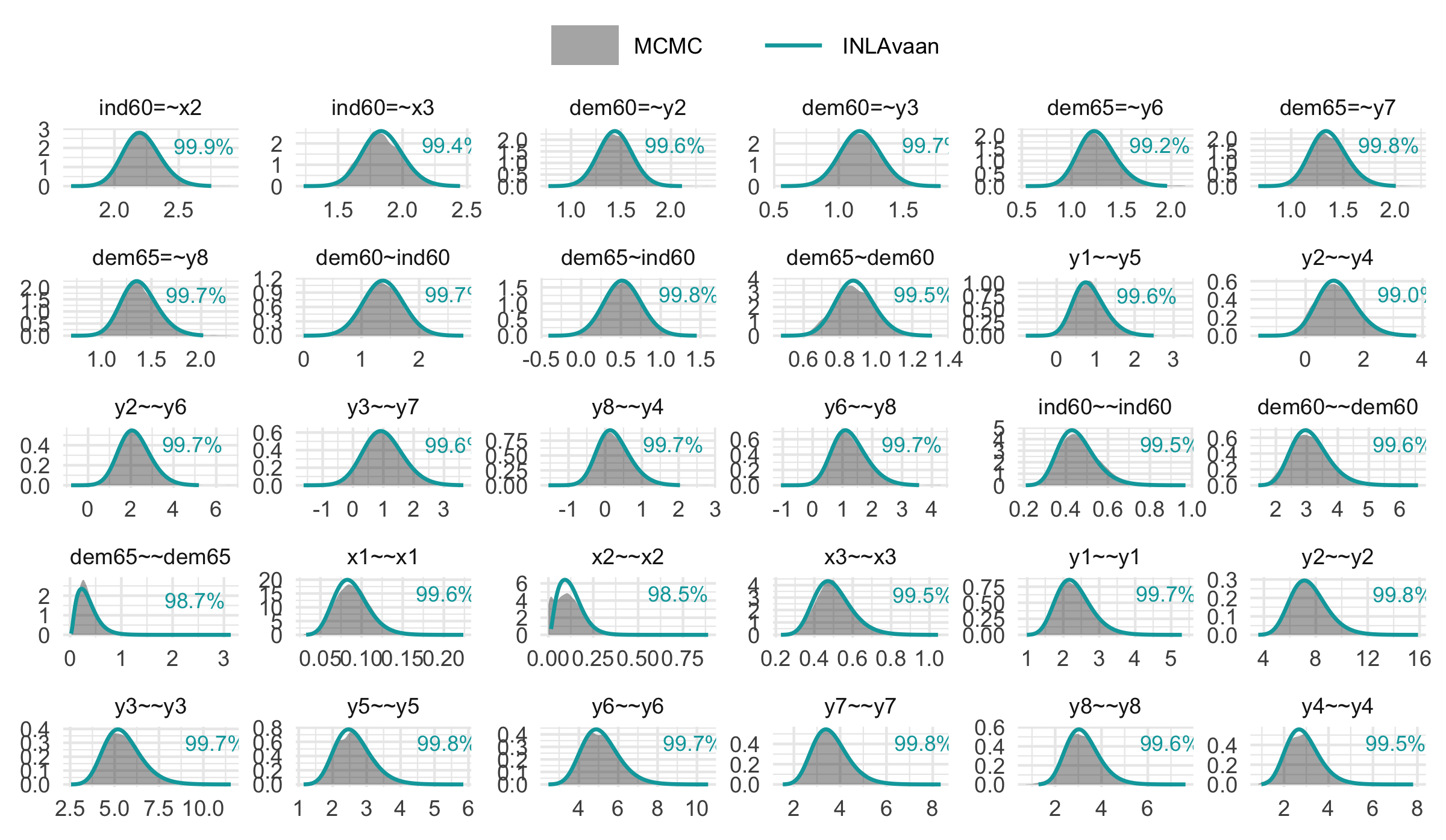
Install the CRAN version of {INLAvaan} using:
install.packages("INLAvaan")Alternatively, install the development version of
{INLAvaan} from GitHub using:
# install.packages("pak")
pak::pak("haziqj/INLAvaan")Optionally2, you may wish to install INLA. Following the official instructions given here, install the package by running this command in R:
install.packages(
  "INLA",
  repos = c(getOption("repos"),
            INLA = "https://inla.r-inla-download.org/R/stable"),
  dep = TRUE
)To cite package {INLAvaan} in publications use:
Jamil, H (2026). INLAvaan: Approximate Bayesian Latent Variable Analysis. R package version 0.2.3. DOI: 10.32614/CRAN.package.INLAvaan
A BibTeX entry for LaTeX users is:
@Manual{,
    title = {INLAvaan: Approximate Bayesian Latent Variable Analysis},
    author = {Haziq Jamil},
    year = {2026},
    note = {R package version 0.2.3},
    url = {https://inlavaan.haziqj.ml/},
    doi = {10.32614/CRAN.package.INLAvaan}
}The {INLAvaan} package is licensed under the GPL-3.
INLAvaan: Bayesian Latent Variable Analysis using INLA
Copyright (C) 2026 Haziq Jamil

This program is free software: you can redistribute it and/or modify
it under the terms of the GNU General Public License as published by
the Free Software Foundation, either version 3 of the License, or
(at your option) any later version.

This program is distributed in the hope that it will be useful,
but WITHOUT ANY WARRANTY; without even the implied warranty of
MERCHANTABILITY or FITNESS FOR A PARTICULAR PURPOSE.  See the
GNU General Public License for more details.

You should have received a copy of the GNU General Public License
along with this program.  If not, see <http://www.gnu.org/licenses/>.
By using this package, you agree to comply with both licenses: the GPL-3 license for the software and the CC BY 4.0 license for the data.
Bollen, K. A. (1989). Structural equations with latent variables (pp. xiv, 514). John Wiley & Sons. https://doi.org/10.1002/9781118619179↩︎
R-INLA dependency has been removed temporarily from v0.2.0.↩︎